
Simple Linear Regression
We can express the behavior of several things around nature based on their relationships. There are several types of relationships between things, some of them could describe how to phenomenons are possibly linked, and some of them could be useful to understand the particular interaction between occurrences or situations. This interaction could produce most of the time outcomes or predictions.
Predictions are based in the intuitive and mathematical relation between what is already known and what is to be estimated. If a practitioner could determinate how what is known today relates to a future event, they could use these insights to help considerably the decision making process of an institute/organization.
Francis Galton was responsible for the use of the term regression. In a famous essay, Galton claimed that, despite the tendency of tall parents to produce tall children and short parents to produce short children, the average height of the children of parents of a given height tended to shift, or “regress,” to the average height of the total population.
Regression analysis deals with the study of the dependence of a variable (dependent variable) on one or more variables (explanatory variables) with the objective of estimating or predicting the population mean or average value of the dependent variable.
Linear Regression with two variables
The first step in determining whether a relationship exists between two variables is to examine the graph of the observed (or known) data. This graph, or plot, is called a scatter plot.
A scatter plot can give us two types of information. First, we can visually identify patterns that indicate that the variables are related. If this happens, we can see what kind of line, or estimated equation, describes this relationship. Second, it gives us an indication about the scale of the variables.
Using R and ggplot a scatter plot could be visualized as follows:
1
2
library(ggplot2)
ggplot(dataset,aes(first_variable, second_variable, color=categorical_variable)) + geom_point()
In Python using the module seaborn and a pandas data frame we can plot the scatter plot of two variables as follows:
1
2
3
import seaborn as sns
# dataset should be a pd.DataFrame
sns.scatterplot(data=dataset, x="first_variable", y="second_variable", hue="categorical_variable")
This is an example of a scatter plot for some of the attributes of the dataset mtcars, this dataset is composed by fuel consumption and 10 aspects of automobile design and performance for 32 automobiles (1973–74 models), you can see more information here.

In this case the linear relationship is visible between Miles/(US) gallon (mpg) and Displacement (disp) segregated by the transmission (0: automatic, 1: manual), we can see that if the Miles/gallon increase the displacement of the car decreases. So there is an inverse relation between both variables.
These linear relationships are sometimes not so common in other datasets, an example of this behavior is the following plot of the Corruption vs Democracy index segregated by world region (data extracted from gapminder)

We can see how there is no visual linear relation between both variables.
Regression and correlation
Correlation analysis is closely related to regression analysis, although conceptually the two are very different. In correlation analysis, the main objective is to measure the strength or degree of linear association between two variables.
In regression analysis there is a difference in treatment between the two variables studied that begins with their names: dependent and explanatory variables. A dependent variable is assumed to be statistical, random or stochastic, i.e., it has a probability distribution. In the other hand, we can consider initially that a explanatory variable is fixed (the deterministic component of a model).
Covariance
Covariance indicates the relationship between two quantitative variables. The covariance between the variable “x” and the variable “y” is denoted and calculated as follows:
\[cov(x,y)=\sigma_{xy}=\mathbb{E}[(X-\mu_x)(Y-\mu_y)]\]*This is known as the population covariance
Where $\mu_x$ is the population average for the variable $X$, $\mu_y$ is the population average for the variable $Y$ and $\mathbb{E}$ is a expected value.
In the case of the sample covariance we have the following term:
\[cov(x,y)=\frac{\sum_{i=1}^{n}{(x_i - \bar{x})(y_i - \bar{y})}}{n}\]where $\bar{x}$ and $\bar{y}$ correspond to the sample average for $x$ and $y$ respectively and $n$ is the number of samples
If the covariance value is positive, it indicates that the variables are directly related, i.e. when the values of one variable increase, the values of the other variable also increase. On the other hand, if the value of the covariance is negative, it indicates that the variables are inversely related, i.e. when the values of one variable increase, those of the other decrease.
However, if the covariance between two variables is zero, it indicates that there is no linear relationship between the variables.
The covariance as a measure of the relationship between 2 variables has the following properties:
- It is invariant to changes in the origin of the two variables.
- Depends on unit changes, changing the unit of measurement of both variables changes the covariance.
Calculating the covariance can also be written as follows:
\[S_{xy}=a_{11} - \bar{x}\bar{y}\]Where $a_{11}$ (central mixed moment of order 1,1) has the following forms:
$a_{11}=\frac{1}{N}\sum_{\forall i}{\sum_{\forall j}{x_i y_i n_{ij}}}$, when the observations are aggregated by frequencies
$a_{11}=\frac{1}{N}\sum_{\forall i}{\sum_{\forall j}{x_i y_i}}$ when the observations are NOT aggregated by frequencies
- If the two variables are independent, their covariance is zero.
- The covariance sees a joint comparison between two variables, if it is positive it will give us the information that at high values of one of the variables there is a greater tendency to find high values of the other variable and the other way around for low values in one of the variables. On the other hand, if the covariance is negative, the covariation of both variables will be in the opposite direction: high values will correspond to low values, and low values to high values. If the covariance is zero, there is no clear covariation in either direction. However, the fact that the covariance depends on the variables measurements does not allow comparisons to be made between one case and another.
Correlation
The term correlation is used to denote the existence of a numerical relationship between the variables analyzed. A correlation coefficient expresses quantitatively the magnitude and direction of the relationship between two variables.
Magnitude refers to the closeness of the scatter plot data to a straight line. If the points on the graph are very close to a straight line, the correlation is said to be very strong, while if the points are far from a straight line, the correlation is weak.
Correlation is the degree of linear association between two quantitative variables. If two variables are linearly related, it indicates that a change in the value of one of them will generate a change in the other. To measure the association strength that exists between two variables the Pearson’s coefficient is the most commonly used statistic.
The direction of the linear relationship between the two variables analyzed can be of two types:
- Direct or positive relationship: When as one variable increases, the other variable also increases.
- Inverse or negative relationship: When one variable increases and the other variable decreases. Example: This is the case when analyzing the nominal value of standard vehicles and their years of use; the more years of use, the lower the nominal value.
The correlation calculated using Pearson’s coefficient estimated from the data has the following form:
\[\rho=\frac{\sigma_{xy}}{\sigma_{x}\sigma_{y}}\]where $\sigma_{x}$ and $\sigma_{y}$ are the population variance for $x$ and $y$ respectively and $\sigma_{xy}$ is the population covariance.
The sample Pearson’s coefficient has the following form:
\[\gamma = \frac{cov(x,y)}{s_x s_y}\]where $s_x$ and $s_y$ are the sample variances for $x$ and $y$ respectively.
If the last expression is written in more detail, it has the following form:
\[r_{xy}=\frac{\sum_{i=1}^{n}{w_i(x_i-\bar{x})(y_i-\bar{y})}}{S_X S_Y (\sum{w_i} - 1)}\]where:
- $w_i$ represents expansion factors for each data pair $(x_i, y_i)$ (The expansion factor is a weight that is applied to each study unit in the sample to obtain a population estimate)
- $S_X$ and $S_Y$ are the standard deviations of both variables.
The correlation coefficient has the following properties:
- $r_{xy}$ is always between -1 and 1.
- $r_{xy}$ is positive when there is a positive relationship between both variables.
- $r_{xy}$ is negative when there is an inverse relationship between both variables.
- $r_{xy}$ is close to zero when there is no linear relation between both variables.
By viewing a scatter plot and calculating the correlation coefficient, the following aspects can be determined:
If the coefficient is very close to 1, it is because the points are very close to a straight line with a positive slope. When the coefficient approaches -1, the scatter plot will show the data decaying in an inverse or negative effect (Like in the
mtcarsexample above).If the coefficient is closer to zero it is because the points clustered around the line are not close to it (they are more random), there is no relationship between the variables.
If the coefficient is closer to zero and the scatter plot shows strange shapes, this indicates a clear nonlinear behavior between the variables and it is necessary to use other types of measures to obtain this relationship or transformations in the models.
In R we can compute the correlation between a group of variables using cor(data), for the mtcars example the correlation between mpg and disp is -0.84755, this is a final indication that both variables have an inverse relation. In Python we can use numpy.corrcoef(data_array).
Regression Analysis
If the dependence of a variable with respect to a single explanatory variable is studied, such a study is considered as a simple regression analysis, or two-variable regression analysis. However, if the dependence of a variable is studied with respect to more than one explanatory variable, it is called a multiple regression analysis. In other words, in a two-variable regression analysis there is only one explanatory variable, while in a multiple regression analysis there is more than one explanatory variable.
At first glance we can see from a scatter plot if indeed two variables are related, as a result, we can draw, or “fit” a straight line through our scatter plot to represent the relationship.
When a line is drawn through the points of a scatter plot we are able to identify the degree of association between the variables. The line drawn through the points represents a direct relationship, because $Y$ increases as $X$ increases. If the points are relatively close to this line, we can say that there is a high degree of association between the variable $X$ and the variable $Y$.
For using and calculating simple linear regression models, the following aspects should be taken into account:
- Variable $Y$ is known as the response/dependent variable, this is the variable of interest that was chosen.
Variable $X$ is known as the explanatory/independent variable and this is the one that will attempt to have a direct relationship with the response/dependent variable.
Both the response/dependent variable $Y$ and the explanatory/independent variable $X$ need to be highly correlated in order to expect a good scatter plot showing the linear relationship, if this does not occur there is probably another type of non-linear dependencies not considered by the proposed model.
- In Machine Learning a synonym for these two variables are
target(dependent variable) andfeature(independent variable)
The relationship between variables $X$ and $Y$ can also take the form of a curve. Statisticians call it a curvilinear relationship.
To understand regression models we must go to the simplest step in which there is a possible relationship between two quantitative variables, by painting in a scatter plot the variable $X$ and $Y$ we can fit a line that represents the behavior of the data under a slope and an intercept, this line is known as Simple Linear Regression Line and is written as follows:
\[y=\beta x + \varepsilon\]Where $y$ is an associated term to the dependent variable, $x$ for the independent variable, $\beta$ its associated slope or parameter and $\varepsilon$ the errors of the model which allow to evidence the exactitude with which the model fits the data.
A model can also be expressed as a predictive function as follows:
\[y=f(x_i)\]Where $f$ is intended to show that the variable $y$ is a function of the variable $x$.
After considering all this, some questions arise: How can the beta parameter be estimated? For this it is necessary to understand that the proposed model is considered as a model without intercept; this means that when drawing the regression line through the scatter diagram the beginning of the line will be at the coordinate (0,0) of the Cartesian plane.
In general cases, models with intercept are more commonly used since the behavior of the data does not always follow a straight line pattern starting at the origin, for the case in which it is necessary to draw a regression line with intercept, the following model can be used:
\[y=\beta_0 + \beta_1 x + \varepsilon\]The most common way to calculate the parameter of the simple linear regression is the least squares method.
$y=\beta_0 + \beta_1 x + \varepsilon$ is the model that perfectly fits the population, something that in practice is impossible (we have samples not all data). Thus, this model could be written in terms of expected values such as $\mathbb{E}[Y| X_i] = f(x_i)$ or $\mathbb{E}[Y | X_i] = \beta_0 + \beta_1 x_i$, so we use the following model known as (sample regression function) with similar notation to show what we want to estimate:
\[\hat{y}=\hat{\beta}_0 + \hat{\beta}_1 x + \hat{\varepsilon}\]In terms of matrix notation, this expression can be seen as follows:
\[\begin{bmatrix} y_{1}\\ \vdots \\ y_{n} \end{bmatrix} =\begin{bmatrix} 1 & x_{11}\\ \vdots & \vdots \\ 1 & x_{1n} \end{bmatrix}\begin{bmatrix} \beta _{0}\\ \beta _{1} \end{bmatrix} +\begin{bmatrix} \varepsilon _{1}\\ \vdots \\ \varepsilon _{n} \end{bmatrix}\]We use the symbol “hat” (ex. $\hat{y}$) to represent the individual values of the estimated points, i.e., those points that are on the estimated line.
Variables linearity
Linearity refers to the point at which the conditional expectation of $Y$ is a linear function of $X_i$ in a population model. Geometrically, the regression curve in this case is a straight line. In this interpretation, a regression function such as $\mathbb{E}[Y | X_i] = \beta_0 + \beta_1 x^2_i$ is not a linear function because the variable $x$ is squared.
Parameters linearity
The second interpretation of linearity is produced when $\mathbb{E}[Y | X_i]$ is a linear function of the parameters $\beta$, such as $\mathbb{E}[Y | X_i] = \beta_0 + \beta_1^2 x_i$, which is non-linear with respect to $\beta_1$. This case is an example of a non-linear regression model (in the parameter).
Parameter estimation
For the parameter estimation in linear regression models, in general, the most widely known estimation method is called Ordinary Least Squares Method (OLS).
In the case of the model with intercept, the following reasoning is used to estimate $\hat{\beta}_1$ and $\hat{\beta}_0$:
We estimate $\hat{\beta}_1$ as follows:
\[\hat{\beta}_1 = \frac{\sum{xy}-n\bar{x}\bar{y}}{\sum{x^2} - n\bar{x}^2}\]simplified it can also be written as:
\[\hat{\beta}_1 = \frac{\sum{(x_i -\bar{x})(y_i -\bar{y})}}{\sum{(x_i - \bar{x})^2}}=\frac{S_{xy}}{S_{xx}}\]Then the intercept $\hat{\beta}_0$ can be calculated as follows:
\[\hat{\beta}_0=\bar{y} - \hat{\beta}_1 \bar{x}\]where $\hat{\beta}_0$ represents the expected value in $Y$ when $X$ is equal to zero and $\hat{\beta}_1$ represents the variation in $Y$ when $X$ increases in one unit (the derivative of $Y$ w.r.t $X$)
Ordinary Least Squares properties
The ordinary least squares method is attributed to Carl Friedrich Gauss, a German mathematician. The least squares method has very attractive statistical properties that have made it one of the most effective and popular methods of regression analysis. Lets have a look to the principles behind this estimation technique.
Considering the regression model:
\[y=\hat{\beta}_0 + \hat{\beta}_1 x + \hat{\varepsilon}\] \[=\hat{y} + \hat{\varepsilon}\]where
\[\hat{\varepsilon}=y -\hat{y}\] \[\hat{\varepsilon}=y - \hat{\beta}_0 + \hat{\beta}_1 x_i\]These residuals correspond to the vertical distances between the values that did not fit the model and the regression line, in order to identify if the proposed model is good, it is necessary to check if the amount of errors is close to zero computing the following total distance:
\[S = \sum_{i=1}^{n}{\hat{\varepsilon}_i}\] \[S=\sum_{i=1}^{n}{\hat{\varepsilon}_i}=\sum_{i=1}^{n}{(y_i - \hat{y}_i)^2} = \sum_{i=1}^{n}{(y_i - \hat{\beta}_0 + \hat{\beta}_1 x_i)^2}\]Then the objective is minimize this distance, also named as the sum of squares $S$ of the difference between the observed dependent variable and the predictions given by the linear function.
The estimators obtained above ($\hat{\beta}_0$ and $\hat{\beta}_1$) are known as least squares estimators, since they are derived from the ordinary least squares principle. These estimators have two types of properties:
Numerical properties: Those that hold as a consequence of using ordinary least squares, regardless of how the data were generated.
Statistical properties: Those that hold only with certain assumptions about the way the data were generated.
These different properties can be further described as follows:
OLS estimators are expressed only in terms of the quantities (i.e., $X$ and $Y$ ) observable (i.e., samples).
They are point estimators: Given the sample, each estimator provides only one (point) value of the relevant population parameter (not an interval).
Once the OLS estimators of the sample data are obtained, the sample regression line is obtained without farther calculations, this line has the following properties:
Passes through the sample means of $Y$ and $X$. As $\bar{y} = \hat{\beta}_0 + \hat{\beta}_1 \bar{x}$
The mean value of the estimated $Y$ ($\hat{y}_i$) is equal to the mean value of the real $Y$ for:
\[\hat{y}_i=\hat{\beta}_0 + \hat{\beta}_1 x_i\] \[=(\bar{y} - \hat{\beta}_1 \bar{x}) + \hat{\beta}_1 x_i\] \[=\bar{y} + \hat{\beta}_1 (x_i - \bar{x} )\]When adding both sides of the last equality over the sample values and dividing by the sample size $n$, we obtain:
\[\bar{\hat{y}}=y\]The average of the residuals is 0.
\[-2\sum_{i=1}^{n}{y_i - \hat{\beta}_0 + \hat{\beta}_1 x_i}=0\]However, as $\hat{\varepsilon}_i= y_i - \hat{\beta}_0 + \hat{\beta}_1 x_i $, the last equation gets reduced to:
\[-2\sum_{i=1}^{n}{\hat{\varepsilon}_i}=0\]The expression $y=\hat{\beta}_0 + \hat{\beta}_1 x + \hat{\varepsilon}$ could be defined in a way $X$ and $Y$ are expressed as deviations of their means. for such purpose, we can sum the equation in both sides as follows:
\[\sum{y}=n \hat{\beta}_0 + \hat{\beta}_1 \sum{x_i} + \sum{\hat{\varepsilon}_i}\]when diving by $n$ we obtain:
\[\bar{y} = \hat{\beta}_0 + \hat{\beta}_1 \bar{x}\]where, subtracting $y_i = \hat{\beta}_0 + \hat{\beta}_1 x_i + \hat{\varepsilon}_i$, we can obtain:
\[y_i - \bar{y} = \hat{\beta}_1 (x_i - \bar{x} ) + \hat{\varepsilon}\]or
\[y_i = \hat{\beta}_1 x + \hat{\varepsilon}\]which as mentioned before, it corresponds to a model without intercept or also called deviation form.
The residuals are not correlated with the predicted value $y_i$.
The residuals are not correlated with $x_i$.
The function lm can be used to estimate the parameters of a linear model using ordinary least squares in R, this function can be used as follows:
1
model = lm(dependent_variable~independent_variable, data=my_dataset)
In Python using LinearRegression from the scikit-learn module:
1
2
3
from sklearn.linear_model import LinearRegression
model = LinearRegression()
model.fit(independent_variable, dependent_variable)
To view the estimated parameters in R use the function summary(model) or directly in the form model$coefficients.
In Python the LinearRegression object does not contain a built-in model summary as in R, however we can still see the coefficients using the model.coef_ method. Note: There are some solutions to see the model summary in detail using additional modules, you can have a look to this thread.
Variance analysis
After constructing the parameter estimates, the question to be answered is: Does the variable $X$ have a significant effect on $Y$?
By a statistically significant effect we mean an effect that is large enough to be considered statistically different from zero. In order to give an answer to this question, it is necessary to consider the following hypothesis:
\[H_0=\beta_1=0\] \[H_a=\beta_1\neq 0\]Which can be judged using statistical tests taken from the analysis of variance table.
An analysis of variance table divides the variance of $Y$ into two parts:
- A part related to the contribution of $X$ to $Y$.
- A part related to the contribution of the residuals of the model
Using this table we can understand if the contribution of the variable $X$ is larger than the contribution of the residuals of the model $\varepsilon$.
Visually, an analysis of variance table looks like this:
| Causes of variation | Degrees of freedom | Sum of Squares | Mean Squares | F statistic | P-value |
|---|---|---|---|---|---|
| Model | 1 | $SSR$ or $ESS$ | $MSR$ | ||
| Error (residuals) | n-2 | $RSS$ | $MSE$ | ||
| Total | n-1 | $TSS$ |
The total variability of $Y$ can be expressed as sum between a part explained by the model and a second part associated to the error, this is is represented as follows:
\[\sum_{i=1}^{n}{(y_i - \bar{y})^2} = \sum_{i=1}^{n}{(\hat{y}_i - \bar{y})^2} + \sum_{i=1}^{n}{\varepsilon^2_i}\]The first part is known as the total sum of squares TSS and the second as the explained sum of squares (sum of squares of the model) plus the sum of squares of the error SSE+SSR.
Following the notations in the table, the mean squares are constructed by dividing each sum of squares by their respective degrees of freedom, while the F-statistic has the form:
\[F=\frac{\text{explained variance}}{\text{unexplained variance}}=\frac{MSR}{MSE}\]where $MSR$ refers to the “regression mean square” and $MSE$ is the “mean square error”. This statistic follows an $F$ distribution with 1 degree of freedom in the numerator and $n-1$ degrees of freedom in the denominator.
This statistic is the one used to test the hypothesis of statistical significance on $\beta_1$. That is, if for a simple linear regression model, the value calculated for $F$ is greater than the percentile of the $F$ distribution with $(1 ; n-2)$ degrees of freedom for an established error level $\alpha$, then the null hypothesis is rejected and it is concluded that variable $X$ does have a significant effect on variable $Y$.
Or analogously, one can read the p-value as usual, if the p-value is less than $\alpha$, the null hypothesis is rejected and one concludes that the variable $X$ does have a statistically significant effect on $Y$.
Goodness of fit
We can compute some metrics to evaluate the performance of our model. In the case of linear regression, the coefficient of determination or R-Squared (R2) is used as a measure to quantify the variability of $Y$ explained by the model. The higher the coefficient the better the model explains reality.
In the case of simple linear regression, it coincides with the square of Pearson’s correlation coefficient.
\[R^2 = \frac{\sigma_{xy}^2}{\sigma_{x}^2 \sigma_{y}^2}\]This coefficient is between 0 and 1.
It can also be written as:
\[R^2 = \frac{SSR}{TSS}\]Where $SSR$ is the “sum of squares due to regression” (also called explained sum of squares ESS) and $TSS$ is the “total sum of squares”
The coefficient of determination has the following characteristics:
- $R^2$ values close to 1 will indicate a good fit of the model to the data.
- In general, $R^2$ values close to 0 will indicate a poor fit of the model to the data. However, this depends on the study, in some statistical and machine learning studies finding $R^2$ values of 1% is common due to the nature of the dependent variable. For example, this is frequent when the objective is analyzing/predicting human behavior (human behavior is highly unpredictable).
Example:
Imagine training/fitting a linear regression to detect brain age with an $R^2$ of 78%. This means the variability of brain age is explained in 78% by the model
In Python to get the $R^2$ we can use r2_score from sklearn.metrics as follows:
1
2
3
4
5
6
7
from sklearn.linear_model import LinearRegression
from sklearn.metrics import r2_score

model = LinearRegression()
model.fit(X, y) # X are the features/ independent variable(s)
y_pred = model.predict(X)
r2_score(y, y_pred)
In R we can simply call summary(model)$r.squared
Statistical assumptions
There are several statistical assumptions to consider when fitting a simple linear model:
Linearity:
As mentioned previously, there should be a linear existent relation between $X$ and $Y$, so we can create what we call linear regression:
\[f(x) = \beta_0 + \beta_1 x\]Normality:
The residuals of a model follow a normal distribution, this means that for the i-th observation the error is assumed as normally distributed:
\[\varepsilon_i \sim N(0, \sigma^2)\]Homogeneity:
The expected value of the residuals is zero,
\[\mathbb{E}[\varepsilon_i]=0\]Homoscedasticity
The variance of the residuals is constant, which means the dispersion of the data should be constant
\[VAR(\varepsilon_i) = \sigma^2\]Independency
the observations should be independent,
\[\mathbb{E}[\varepsilon_i \varepsilon_j]=0\]This means one observations should not give information about the others (This is a missing characteristic in time series data, as past observations are linked to future observations)
Parameter inference
Once we estimate the parameters of a simple linear model we are also interested in having a measure of precision on those estimates to verify whether the calculated values could be the true values for our parameters. This can be done by statistical inference.
To do so, we can create and test the following statistical hypotheses:
\[H_0: \beta_0 = 0\] \[H_a: \beta_0 \neq 0\]and
\[H_0: \beta_1 = 0\] \[H_a: \beta_1 \neq 0\]Contrasting these hypotheses implies calculating the next test statistic:
\[t=\frac{\hat{\beta}_i}{\sqrt{\hat{VAR}(\hat{\beta}_i)}}\]This statistic follows a $t$-distribution with $n-2$ degrees of freedom. This means that the null hypothesis is rejected at the $\alpha$ level of significance if the absolute value of the statistic is greater than the $\alpha /2$ percentile of the $t$-distribution with $n-2$ degrees of freedom. Or analogously, when the calculated p-value is less than $\alpha$.
But how can we compute this statistic?
The first thing to know is that both $\beta_0$ and $\beta_1$ are also random variables and both follow a normal distribution since both are produced by linear combinations of normals. To prove this we can rewrite the expressions to compute the estimations as follows:
For the slope parameter:
\[\hat{\beta}_1 = \frac{\sum{(x_i -\bar{x})(y_i -\bar{y})}}{\sum{(x_i - \bar{x})^2}}=\frac{\sum{(x_i -\bar{x})}Y_i}{\sum{(x_i - \bar{x})^2}}\]This last expression is produced using the equivalence:
\[S_{xy}=\sum{(x_i -\bar{x})(y_i -\bar{y})}=\sum{(x_i -\bar{x})}y_i\]For the intercept parameter:
\[\hat{\beta}_0=\bar{Y} - \hat{\beta}_1 \bar{x}\]
As both expressions are written in terms of $Y_i$, where $Y_i \sim N(\beta_0 + \beta_1 x_i, \sigma^2)$, using the properties of expected value and variance, we can find the normal distributions of both parameters:
\[\hat{\beta}_1 \sim N \left(\beta_1, \frac{\sigma^2}{(n-1)S_{xx}} \right)\] \[\hat{\beta}_0 \sim N\left(\beta_0, \sigma^2 \left( \frac{1}{n} + \frac{\bar{x}^2}{(n-1)S_{xx}}\right) \right)\]By using these distributions, we can construct confidence intervals for the parameters using the $t$-distribution. These have the following form:
\[CI(\beta_0)=\hat{\beta}_0 \pm t_{\frac{\alpha}{2}, n-2}\sqrt{\hat{VAR}(\hat{\beta}_0)}\] \[CI(\beta_1)=\hat{\beta}_1 \pm t_{\frac{\alpha}{2}, n-2}\sqrt{\hat{VAR}(\hat{\beta}_1)}\]Usually these statistics are computed automatically in libraries and modules in R and Python.
In R using the following lines will give you all sorts of information about the model:
1
2
model = lm(y~x)
summary(model)
In Python we can compute all statistics by hand after computing the coefficients using scikit-learn or simply use the module statsmodels as follows:
1
2
3
import statsmodels.api as sm
model_results = sm.OLS(y, x).fit()
print(results.summary())
Practical example
After all of this dense mathematical introduction, let me show an example.
In this case I am going to use R exclusively, since it is more convenient for this case in which we are trying to understand statistical concepts.
I always recommend using R when the task is exclusively based on statistical data analysis and using Python for machine learning tasks. This is because R offers a variety of built-in statistical methods that are quite useful when working with linear models or statistical tests.
However, it depends on the preferences and tasks of the practitioner; if you are fitting a linear model and your interest is to generalize over a test set, you may always find it more convenient to use modules such as scikit-learn, Tensorflow or PyTorch in Python.
In this case we will be using the dataset diamonds from ggplot2. This is a dataset containing the prices and other attributes of almost 54,000 diamonds.
This is how we can start loading the data and plotting some interesting descriptive statistics
1
2
3
4
5
6
# It is a good coding practice to import your libraries on the top of the code!
library(ggplot2)

# Load the data and generate a descriptive statistics summary
data = as.data.frame(diamonds)
summary(data)
     carat               cut        color        clarity          depth           table           price             x
 Min.   :0.2000   Fair     : 1610   D: 6775   SI1    :13065   Min.   :43.00   Min.   :43.00   Min.   :  326   Min.   : 0.000
 1st Qu.:0.4000   Good     : 4906   E: 9797   VS2    :12258   1st Qu.:61.00   1st Qu.:56.00   1st Qu.:  950   1st Qu.: 4.710
 Median :0.7000   Very Good:12082   F: 9542   SI2    : 9194   Median :61.80   Median :57.00   Median : 2401   Median : 5.700
 Mean   :0.7979   Premium  :13791   G:11292   VS1    : 8171   Mean   :61.75   Mean   :57.46   Mean   : 3933   Mean   : 5.731
 3rd Qu.:1.0400   Ideal    :21551   H: 8304   VVS2   : 5066   3rd Qu.:62.50   3rd Qu.:59.00   3rd Qu.: 5324   3rd Qu.: 6.540
 Max.   :5.0100                     I: 5422   VVS1   : 3655   Max.   :79.00   Max.   :95.00   Max.   :18823   Max.   :10.740
                                    J: 2808   (Other): 2531
       y                z
 Min.   : 0.000   Min.   : 0.000
 1st Qu.: 4.720   1st Qu.: 2.910
 Median : 5.710   Median : 3.530
 Mean   : 5.735   Mean   : 3.539
 3rd Qu.: 6.540   3rd Qu.: 4.040
 Max.   :58.900   Max.   :31.800
In these statistics we can see a summary of the different characteristics of the 54,000 diamonds in the dataset, including color distribution, average price and carat count. We can then try to find some relationships in the data with scatter plots and correlations.
For this example we are interested in finding the relationship between the price and carat of all diamonds, we can see from the statistics above that the scales for both variables are different, we can re-confirm this visually with the next scatter plot:
1
2
3
# Plot the relationship between carats and price by color
ggplot(data, aes(carat, price, color=color)) + geom_point()
cor(data$carat, data$price)
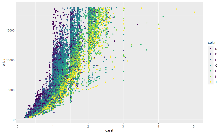
In the plot we can also see the linear trend visually between both attributes, for price and carat the correlation is 0.9215913 which indicates a strong linear relation, this in the end allows us to model the data with linear regression as follows:
1
2
model = lm(price~carat, data = data)
summary(model)
Call:
lm(formula = price ~ carat, data = data)

Residuals:
     Min       1Q   Median       3Q      Max
-18585.3   -804.8    -18.9    537.4  12731.7

Coefficients:
            Estimate Std. Error t value Pr(>|t|)
(Intercept) -2256.36      13.06  -172.8   <2e-16 ***
carat        7756.43      14.07   551.4   <2e-16 ***
---
Signif. codes:  0 ‘***’ 0.001 ‘**’ 0.01 ‘*’ 0.05 ‘.’ 0.1 ‘ ’ 1

Residual standard error: 1549 on 53938 degrees of freedom
Multiple R-squared:  0.8493,	Adjusted R-squared:  0.8493
F-statistic: 3.041e+05 on 1 and 53938 DF,  p-value: < 2.2e-16
We can see in these results the coefficients in the Estimate field and the different statistics that we discussed in the previous sections such as the test statistic t test.
If we look at the p-values of the parameters associated with the intercept and carat, we can say that both are statistically significant as the p-value < 0.05. We can also see how good the goodness of fit of the model is by looking at the $R^2=0.8493$, which means that ~85% of the price variability is explained by the model (In this case is not a great performance, taking into account the characteristics of the dependent variable price).
For the interpretation of the coefficients, we see that the intercept does not have a direct interpretation, because when the carat is 0 the price is -2256 dollars, which does not make any sense. However, we can see for the case of the parameter associated with the explanatory variable that as the carat increases by one unit, the price increases by 7756.43 dollars.
We can take a look at the statistical significance of the parameters with the analysis of variance of the model using anova(model). This line will give the following results:
Analysis of Variance Table

Response: price
             Df     Sum Sq    Mean Sq F value    Pr(>F)
carat         1 7.2913e+11 7.2913e+11  304051 < 2.2e-16 ***
Residuals 53938 1.2935e+11 2.3980e+06
---
Signif. codes:  0 ‘***’ 0.001 ‘**’ 0.01 ‘*’ 0.05 ‘.’ 0.1 ‘ ’ 1
This is a representation of the highlighted table discussed in the Analysis of Variance section containing all the aforementioned statistics, where in this case the p-value <0.05 indicates the carat explains the diamond price and it is a necessary explanatory variable in our final model.
The final linear model equation could be written as follows:
\[\hat{price} = -2256.36 + 7756.43 (carat)\]We can use this equation by substituting carat for a given quantity to make some predictions.
Note that further analysis of this model is required to know if it is good enough to explain the desired relationship. This involves analyzing the residuals to verify that our model works correctly and follows the statistical assumptions we mentioned previously. This is going to be investigated using some additional statistical tests and plots in a new another post.
Cite:
1
2
3
4
5
6
7
@misc{LinearModels101Intro,
  author = {Miguel A. Alba},
  title = {Linear models 101! - Introduction: Simple Linear Regression},
  year = 2021,
  url = {https://miguelalba96.github.io/posts/LinearModels-intro},
  urldate = {2021-10-14}
}